前面介绍过线性回归,并使用了R语言实现了训练模型,完成了通过水的沸点来估计海拔高度的预测。链接
R语言封装了最小二乘法的具体实现。我们在调用时对其内部细节感触并不是很深,下面使用python实现 最小二乘法,加深对模型训练的理解。
0.导入数据
我们还是用前面准备好的数据,保存成a.csv
1
2
3
4
5
6
7
8
9
10
11
12
13
14
15
16
17
| 194.5,131.79
194.3,131.79
197.9,135.02
198.4,135.55
199.4,136.46
199.9,136.83
200.9,137.82
201.1,138.00
201.4,138.06
201.3,138.05
203.6,140.04
204.6,142.44
209.5,145.47
208.6,144.34
210.7,146.30
211.9,147.54
212.2,147.80
|
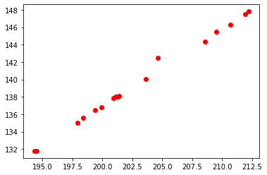
编写python的numpy和matplotlib.pyplot,读取a.csv并且画出所有点
1
2
3
4
5
6
7
8
9
10
11
| import numpy as np
import matplotlib.pyplot as plt
f = '/tmp/a.csv'
array = np.genfromtxt(f,delimiter=',')
x = array[:,0]
y = array[:,1]
plt.scatter(x,y,c='r')
plt.show
|
1.实现算法
下面定义一个fit方法,实现模型训练。
1
2
3
4
5
6
7
8
9
10
11
12
13
14
15
16
17
18
|
def fit(x,y):
sum_xy = 0
sum_x = 0
sum_y = 0
sum_x2 = 0
n = x.shape[0]
for i in range(n):
sum_xy += x[i]*y[i]
sum_x += x[i]
sum_y += y[i]
sum_x2 += x[i] ** 2
a = ((sum_xy/n) - (sum_x/n) * (sum_y/n)) / ((sum_x2/n) - (sum_x/n) * (sum_x/n))
b = (sum_y/n) - (a * (sum_x/n))
return a,b
|
为了方便看误差,我们定义计算损失函数
1
2
3
4
5
6
7
8
9
10
11
12
| def compute(a,b,points):
x = points[:,0]
y = points[:,1]
pred_y = a * x + b
n = y.shape[0]
total = 0
for i in range(n):
total += math.fabs(y[i] - pred_y[i])
return total
|
2.测试
1
2
3
4
5
6
7
8
9
10
11
12
13
14
15
16
|
a,b = fit(x,y)
cost = compute(a,b,array)
print("a is: ", a)
print("b is: ", b)
print("cost is: ", cost)
plt.scatter(x,y,c='r')
pred_y = a * x + b
plt.plot(x,pred_y,c='b')
plt.show()
|
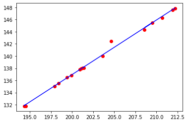
我们发现算出来的斜率是0.8954625247967952,截距是-42.130870767876615
与R已封装的包,算得的结果很接近,这也证明了写的代码没啥问题!